Classification Evaluation Metrics
Classification Evaluation Metrics
I trained a model and got 99% accuracy on training! Whoopie! That is the general reaction of mostly all beginners when they come across training neural networks, and simple classification tasks. However, from a standard or industrial point of view, getting a high training accuracy is not the end goal rather making an adaptive classification model robust to outliers, and unseen data is the target which is suitable for deployment.
A model’s ability is not measured by how well it memorizes training data, rather it is measured by how well it generalizes on test data, or unseen new instances. A model should not memorize features, it would lead to over-fitting on training data and is not an ideal situation. Also, on the contrary, a model should not learn a very few features either that may lead to under-fitting on the data and hence, result in poor performance as well.

As shown above, a balanced model will be able to fit most of the data points and should be robust to new data points that may be fed to it. The model is underfitting the training data when the model performs poorly on the training data. This is because the model is unable to capture the relationship between the input instances and the target values. The model is overfitting the training data when you see that the model performs well on the training data but does not perform well on the evaluation data. This is because the model is memorizing the data it has seen and is unable to generalize on unseen examples.
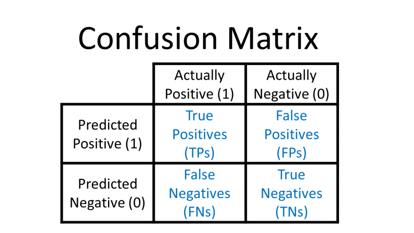
We specifically concentrate on evaluating classification tasks in supervised learning problems where we need to assign a label to each data point (or rather to assign the target class Y to each input instance X correctly). This can have the following scenarios:
- True Positive (TP): The data point was actually true and correctly classified as true by the model.
- False Positive (FP): The data point was actually true and incorrectly classified as false by the model.
- True Negative (TN): The data point was actually false and correctly classified as false by the model.
- False Negative (FN): The data point was actually false and incorrectly classified as true by the model.
Let us try to understand this as an example of credit card fraud transaction classification task.
Task (T): To classify each transaction as legitimate or fraud Target/Labels (Y): Legitimate or Fraud
So, given a set of input features we need to assign labels to each transaction as fraud or legitimate. Let us get to the different varieties of evaluation metrics.
 For this we have,
- True Positive: A legitimate transaction classified as a legitimate transaction by the model.
- True Negative: A fraud transaction correctly classified as a fraud transaction by the model.
- False Positive: A legitimate transaction incorrectly classified as a fraud transaction by the model.
- False Negative: A fraud transaction incorrectly classified as a legitimate transaction by the model.
Now, in this case, Case 3 and Case 4 are the errors made by the model in classification task T. However, Case 4 proves to be more fatal than Case 3. Consider from the point of view of a bank, a legitimate transaction being classified as fraud can be verified by the user with a discussion and evidence provided to the bank by them. However, in case a fraud transaction is classified as a legitimate transaction then this will cost the bank much more resources. Thus, a robust or rather a desirable model will be one which may have some false positives but should not have any false negatives at all. Hence, as we see from a real-life application point of view, we need not be perfect but should suitably serve the needs of a specific task.
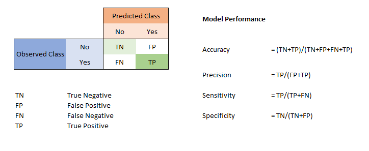
From this matrix, we come to the following metrics suitable for evaluation:
- Accuracy: (True Positives/True Positives+True Negatives+False Positives+False Negatives)
- Precision: (True Positives/True Positives+False Positives)
- Recall or Sensitivity: (True Positives/True Positives+False Negatives)
- Specificity: (True Negatives/True Negatives+False Positives)
 Now, we need to understand what all these metrics indicate in evaluating a model.
- Accuracy indicates the proportion of correct classification in all the possible classified instances. Hence, it is a good measure when each class or target variable has equal number of instances that is for example the number of fraud transaction is same as the number of legitimate transactions.
- Precision: It is the fraction of relevant instances among the retrieved instances. It gives a measure of “how often” the model is correct. It is (TP/Predicted Positives) in simple terms.
- Recall: It is the fraction of relevant instances among the actual number of retrieved instances. It gives the idea of “how often” it predicts correctly when it is actually correct. It is (TP/Actual Positives) in simple terms. Thus, it describes how sensitive the model can be to the actual data.
- Specificity: Specificity relates to the classifier’s ability to identify negative results. Consider the example of medical test used to identify a certain disease. The specificity of the test is the proportion of patients that do not to have the disease and will successfully test negative for it.
There is a trade-off between the precision and recall with the goal of maximizing both of them. However, if we increase precision then recall decreases and vice versa. So, it depends on the application or use case for which we are training the model. For example as discussed above, credit card transactions can tolerate false positives to a degree but cannot work with false negatives at all, hence we need to maximize recall for it.
Thus, we require a metric that can be used to balance between precision and recall to a good degree. So, we make use of a metric called F1-Score which is the harmonic mean of precision and recall for a classification problem.
F1-Score
F1 Score = (2*Precision*Recall)/(Precision+Recall)
Now comes the question why we take the harmonic mean, and how it is better than taking an arithmetic mean. So, the simple answer to this is that harmonic mean punishes extreme values much more than arithmetic mean. Let us observe the following scenarios:
-
Precision=0 and Recall=1: F1 Score = (2 * 0 * 1)/(2 + 0) = 0 However, if we use arithmetic mean then we get 0.5 which is a decision value for a classifier and can imply the possibility of both the classes.
-
Precision=1 and Recall=0: Again, F1 Score = 0 and if we use arithmetic mean then it will be 0.5 so it is indicating both classes equally which is pretty irrelevant for a classifier.
It tells you how precise your classifier is (how many instances it classifies correctly), as well as how robust it is (it does not miss a significant number of instances).
High precision but lower recall, gives you an extremely accurate, but it then misses a large number of instances that are difficult to classify. The greater the F1 Score, the better is the performance of our model.
Also, sometimes, we make use of weights attached to precision and recall for tuning purposes.
It makes it more effective in evaluating a model.

ROC Curve
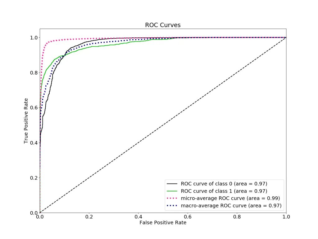
A receiver operating characteristic curve is a graphical plot between the true positive rate (TPR) versus the false positive rate (FPR) as a threshold of being positive on an instance being varied.
True Positive Rate (TPR) is a synonym for recall and is therefore defined as follows:
TPR = (True Positives/True Positives+False Negatives)
False Positive Rate (FPR) is defined as follows:
FPR = (False Positives/False Positives+True Negatives)
Hence, the TPR gives us a sense of how sensitive is the data, and the FPR gives us the sense of how often the model classifies incorrectly.
Steps to Generate ROC Curve
- Sort the test predictions according to the confidence that each prediction is positive.
- Step through the sorted list from high confidence to low
- Locate a threshold between instances of opposite classes, keeping in mind that the instances with same confidence value should be on the same side of the threshold
- Compute TPR, FPR and output them on the plot graphically as FPR vs TPR The goal is obviously to maximize the TPR and minimize the FPR.
ROC Curve is insensitive to changes in class distribution and even if the proportion of positive to negative instances changes in a test set, the ROC curve will not be affected by it. This is called Class Skew Independence. This is because the metrics TPR and FPR used for ROC are independent of the class distribution as compared to other metrics like accuracy, precision, etc., which are impacted by imbalanced class distributions.
Area under the ROC Curve (AUC)
AUC measures the entire two-dimensional area underneath the entire ROC curve from (0,0) to (1,1). AUC provides an aggregate measure of performance across all possible classification thresholds. One way of interpreting AUC is as the probability that the model ranks a random positive example more highly than a random negative example. Higher the AUC value, better is the model. AUC is desirable for the following two reasons:
- AUC is scale-invariant. It measures how well predictions are ranked, rather than their absolute values.
- AUC is classification-threshold-invariant. It measures the quality of the model’s predictions irrespective of what classification threshold is chosen.
However, it only takes into account the order of probabilities and hence it does not take into account the model’s capability to predict higher probability for samples more likely to be positive. Hence, it is useful to only see how the model is able to distinguish between two classes

ACKNOWLEDGMENTS
- ANALYTICSVIDHYA
- MEDIUM
- FRITZ AI
- GOOGLE MACHINE LEARNING CRASH COURSE